7 Employee Lifetime Value

The concept of lifetime value (LTV) is widely applicable across multiple fields. It is used to measure the total value or contribution that a specific entity (e.g., customer, subscriber, employee) brings to an organisation over the expected tenure of their engagement with the organisation. Many would be familiar with customer lifetime value in marketing but in this chapter I will detail how actuarial methods can be used to estimate ELTV.

7.1 Employee Value over Time (ELTV)

The value an employee brings to an organisation is determined by many factors including:

• Their direct financial contributions in revenue generation or cost savings
• Their output and quality of work.
• Skills and expertise such specialised knowledge or the ability to make decisions.
• Intangible contributions such as initiative, innovation, upskilling, EQ and their alignment with the company culture
• Loyalty and reliability (if high performing).

The cost to the company to have that employee also has many factors including:

• Contractual direct costs including salary, benefits provided and paid leave
• Government mandated employment costs like employer taxes, levies and social security contributions. Some locations may be cheaper for salaries but government costs can offset much of the savings
• Indirect costs such as perks, insurance, overhead costs, training and development and equipment and workspace costs
• Recruitment costs: The initial acquisition cost of an employee
• Exit costs: The loss in revenue as a result of the employee leaving
• Opportunity costs: The missed revenue as a result of the employee not performing to or exceeding expectations.

The graph above showcases a simple but exaggerated view of employee value over time. Every given point in time corresponds to the value the employee has brought to the organisation. So, for example, at time 5, the employee has cost the company around 40000. At time 28, they have now broken even and “paid back” their initial costs and ramp up time. At time 90 they have brought in the maximum value they can.

In this simplistic example, we see an employee who:

• Has an upfront acquisition cost
• Takes a few months to ramp up incurring further costs
• Begins to understand the business requirements and deliver value
• Remains an average performer over their lifetime
• Becomes a bit stale in their role due to lack of upskilling and the changing nature of the role
• The market value of the role reduces due to automation or other factors but the employee continues to earn a salary based on the original value of the role
• The employee eventually generates negative value as their cost is much higher than the output produced

If we look at the expected future value to be brought in over the next 2 years, we see the following:

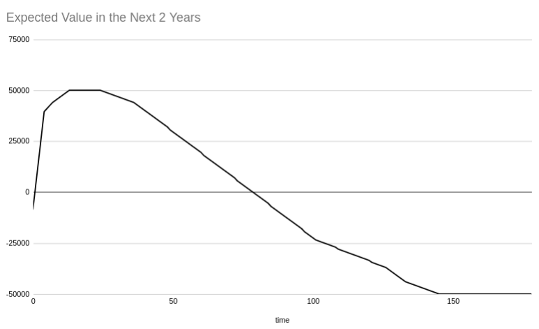
Figure 3.1: ELTV Example 2

Up to time ~80, the employee is still expected to return value in the next 2 years. We can see that after the initial ramp up, the employee is expected to generate value for quite a long period. These simple charts provide some “obvious” actions when trying to maximise employee value including:

• Reducing acquisition costs
• Minimising ramp up time
• Ensuring compensation is flexible and commensurate with the labour markets
• Ensuring employees are given opportunities to learn new skills and remain relevant in the job market
• Ensuring employees are able to perform at the highest levels of performance
• Knowing when it is time to retrain or retrench an employee who no longer is able to generate value

7.2 Present Value of Future Profits

So, how do we calculate the expected value of an employee? In a life insurance company, the value of a policy is often calculated as the Present Value of Future Profits (PVFP) generated by the policy. This involves projecting all future cash inflows (like premiums) and cash outflows (like claims, benefits, and expenses) and then discounting those future cash flows to the present to account for the time value of money. It is a measure of the economic value of the active business to the shareholders.

The calculation of the value of a policy is based on actuarial principles, and the value depends on various factors like mortality rates, policyholder behavior, expenses, investment returns, and the discount rate.

It is generally defined as: \[ \begin{aligned} \mathrm{Policy\ Value} &= \sum_{t=0}^{n}\frac{(P_t-E_t)\times_tp_x+C_t\times_tq_x}{(1+r)^t}\\ \end{aligned} \] where: \(t\) = the time period (typically in years, from 0 to nn, where nn is the number of periods in which the policy generates cash flows). \(P_t\) = Premiums received in year \(t\). \(_tp_x\) = the probability of surviving to time t \(C_t\) = Claims or benefits paid to policyholders in year \(t\). \(_tq_x\) = the probability of claiming in time t \(E_t\) = Expenses related to the policy (e.g., administrative, acquisition, maintenance expenses) in year \(t\). \(r\) = Discount rate (often based on the company’s cost of capital or the risk-free rate). \(n\) = Expected duration of the policy (number of years over which the policy generates cash flows).

Depending on the business in question, EV can be quite a useful measure especially if the company is interested in long-term workforce and cost planning. In relation to PA, this can be constructed as follows:

\[ \begin{aligned} \mathrm{Employee\ Value} &= \sum_{t=0}^{\infty}\frac{(I_t-E_t)\times_tp_x-L_t\times_tq_x}{(1+r)^t}\\ \end{aligned} \] where: \(t\) = the time period (typically in years, from 0 to \(n\), where \(n\) is the number of periods in which the policy generates cash flows). \(I_t\) = The company income attributable to an employee in time \(t\). \(_tp_x\) = the probability of working to time \(t\) \(L_t\) = Costs directly related to the loss of the employee in time \(t\). \(_tq_x\) = the probability of resigning in time \(t\) \(E_t\) = Expenses related to the employee (e.g., salary, bonuses, benefits, etc) in time \(t\). \(r\) = Discount rate (often based on the company’s cost of capital or the risk-free rate). \(n\) = Expected tenure of the employee (number of years over which the employee generates cash flows).

The formula is quite simple and logical but, the main advantage it gives is that each item can be considered a random variable instead of a fixed value or discrete formula. As a result, various factors can be applied to each item depending on the use case in question.

For example, consider the following situation:

• We have observed in our data that a group of employees experiences a U curve of adjustment over 3 years.
• The employees generate high value in their first year, followed by a reduced value in their second year.
• Thereafter, they are able to return to their initial productivity.
• In their 2nd year of tenure, an employee wishes to leave and has been offered a 10% increase to join another company
• Should we be looking to match this offer to retain the employee?

Assume the following:

\(t\) = 28 \(I_t\) = \(1.5 \times E\) it would have been \(1.65 \times E\) but it needs to be reduced by the counter offer (10%) \(_tp_{28}\) = the probability of working to time \(t\) given that they have worked to time \(28\) \(L_t\) = Costs directly related to the loss of the employee in time \(t\). Let this be \(0.75 \times E\) \(_tq_x\) = the probability of resigning in time \(t\) \(E_t\) = Expenses related to the employee (e.g., salary, bonuses, benefits, etc) in time \(t\). \(r\) = Discount rate. To simplify this example, let \(r = 0\%\) \(n\) = Expected tenure of the employee

We then have \[ \begin{aligned} \mathrm{Employee\ Value} &= \sum_{t=28}^{\infty}\frac{(0.5 \times E_t)\times_tp_{28}-0.75 \times E_t \times_tq_{28}}{(1)^t}\\ \end{aligned} \]

and we know that \(_tp_x = 1 - _tq_x\) giving:

\[ \begin{aligned} \mathrm{Employee\ Value} &= \sum_{t=28}^{\infty}\frac{(0.5 \times E_t)\times(1-_tq_{28})-0.75 \times E_t \times_tq_{28}}{(1)^t}\\ &= \sum_{t=28}^{\infty}-1.25 \times E_t \times _tq_{28} + 0.5 \times E_t\\ &= \sum_{t=28}^{\infty}(-1.25 \times _tq_{28} +0.5)E_t \end{aligned} \]

From this, we can see that we should only match the offer if the sum above is \(>= 0\)

However, we may find that once a counter offer is made, an employee exhibits a different attrition pattern than if they never began interviewing elsewhere. We should use the appropriate decrement rate applicable to employees who’ve received counter offers. If we further assume:

• 5% attrition per month in the next 12 months and,
• 50% attrition per month in the 12 months after that

it would take nearly 5 years for the ELTV to become negative for this employee so a counter offer should be presented.

While this example, I hope you can appreciate how powerful this kind of approach can be when making financial decisions on employees.