8 Valuing Projects

PA professionals often need provide key financial calculations relating to the projects that they’ve done or to show the value of a future project that requires some upfront investment. In the former, it can sometimes feel like a case of justifying why the team exists (and should continue to do so) while in the latter, it’s a case of proving what can be achieved with further investment.

Suppose the finance or executive team are considering the merits of different investment or business projects. These projects usually consist of an upfront cost and potentially more costs in the future. In return, at some future stage, the projects will generate an income (regular or otherwise). All projects can have quite varied structures and risks so, to be able to quantify them is critical to be able to provide decision makers with enough information.

8.1 Cashflow Estimation

The estimation of the cash inflows and outflows associated with a project is a difficult task that combines science, logic and art. It usually requires considerable experience and judgement in order to understand all the cashflows involved as well as all the risks associated with those cashflows. All the relevant factors and risks (such as implementation delays) should be considered by the analyst, with assistance from experts in the relevant field (eg time spent on a manual task to be automated). The identification and assessment of the risks may be conducted using the Risk Analysis and Management for Projects (RAMP) approach for risk analysis and management that has been developed by, and published on behalf of, the actuarial and civil engineering professions. Since there will be uncertainty in the assessment of many of the risks, it is prudent to perform calculations using various scenarios and their associated probabilities. For example, conducting forecasts that are ‘optimistic’, ‘average’, and ‘pessimistic’.

In actuarial terms, the set of optimistic assumptions is often called a ‘weak’ basis and the pessimistic set of assumptions is often called a ‘strong’, ‘prudent’ or ‘cautious’ basis. Average assumptions are also called ‘best-estimate’ or ‘realistic’ assumptions.

Let’s have a look at an example:

Project A:

Initial outlay of $50000
Thereafter, annual fees of $50000 for another 3 years with each year’s payment probability being 85% of the previous years
At the end of year 4, an expected income of $300000 if all previous payments were made, otherwise 0

Project B - Paying a recent graduate a higher salary - Initial outlay of $100000 - Thereafter, annual fees of $100000 at the end of every year for 3 years with each payment probability being 70% of the previous payments - At the end of year 4, an expected income of $800000 with probability at 70% of the previous year’s expenses.

8.2 Net Present Value

If we assume the a discount rate of $5\%$ then the $Net\ Present\ Value\ (NPV)$ of the 2 projects can be calculated as:

\[ \mathrm{NPV\ Project\ A} = -50000 -50000\times1.05^{-1}\times0.85-50000\times1.05^{-2}\times0.85^{2}\\ -50000\times1.05^{-3}\times0.85^{3} + 300000\times1.05^{-4}\times0.85^{3}\\ = 52329.02\\ \]

\[ \mathrm{NPV\ Project\ B} = -100000 -100000\times1.05^{-1}\times0.7-100000\times1.05^{-2}\times0.7^{2}\\ -100000\times1.05^{-3}\times0.7^{3} + 800000\times1.05^{-4}\times0.7^{4}\\ = 44028.98 \]

In this example, Project B is more valuable than project A. If we took account of only the cashflows, project B is the better option. If we took account of only the discount rates then Project B is the better option. If we took account of only the probability of the cashflows occurring, then project B is better. However, all 3 options give the incorrect result.

Another way to confirm this is to look at the $Internal\ Rate\ of\ Return\ (IRR)$ of the 2 projects.

8.3 Internal Rate of Return

The IRR is the discount rate that makes the NPV of a series of cash flows equal to zero. In other words, it’s the rate at which the present value of future cash inflows equals the initial investment cost. The IRR is widely used in finance to evaluate the profitability of investments, especially when comparing different projects or investments.

The formula for calculating IRR is based on the Net Present Value (NPV) equation:

\[ 0 = \sum_{t=0}^{n} \frac{C_t}{(1 + \text{IRR})^t} \]

Where: - $C_t$ = Cash flow at time $t$, - $t$ = Time period (e.g., year), - $n$ = Total number of periods, - $IRR$ = Internal Rate of Return.

To break it down, this equation says that the sum of the present values of all future cash flows should be zero.

If there’s an initial investment of $C_0 = -1000$ (an outflow of 1,000) and future cash flows of $C_1 = 300$, $C_2 = 400$, $C_3 = 500$, we want to find the IRR that satisfies:

\[ 0 = \frac{-1000}{(1 + \text{IRR})^0} + \frac{300}{(1 + \text{IRR})^1} + \frac{400}{(1 + \text{IRR})^2} + \frac{500}{(1 + \text{IRR})^3} \] Unfortunately, IRR cannot be solved directly algebraically in most cases because it’s a non-linear equation with multiple terms. Typically, IRR is found using trial and error, interpolation, or more commonly, using computational methods like the Newton-Raphson method or software tools which have a built-in IRR function.

The 2 projects above return IRRs of 16.76% and 10.29% respectively further cementing Project A as the preferred option.

8.4 Other Considerations

When deciding between investment projects, financial metrics like NPV and IRR provide essential quantitative insights. However, they often fall short of capturing the entire scope of considerations required for a sound decision, especially when values are close or conflicting, or, when external borrowing is involved. In these situations, other qualitative factors come into play including:

Synergies with other projects
Political constraints
Upside potential
Resources

8.5 Detailed Project Appraisal

The cashflows are only a part of a detailed project appraisal. In order to provide a valid and thorough submission, the following is a view of the appraisal process in full with the steps laid out below:

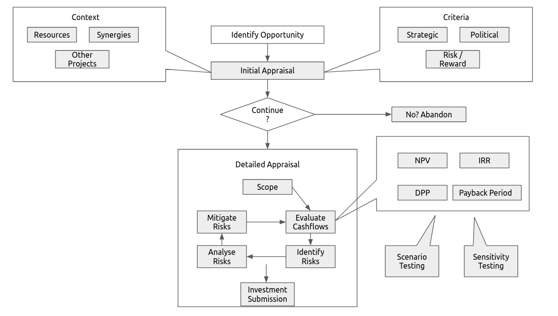
Figure 3.1: Project Appraisal Flowchart

8.5.1 Scope: The detailed definition of the project. This specifies:

Criteria
Timescale
Budget
Responsibilities
Issues that you’re not responsible for

8.5.2 Evaluate Cashflows: This involves quantifying the following:

Capital expenditure
Running costs
Revenues
Termination costs

and then documenting all of these assumptions and the effects they will have. As part of this process, the techniques discussed above will need to used to assess the project and using the cashflows. Sensitivity testing (changing 1 assumption) must be carried out to assess if assumptions are wrong and how the outcome changes with the assumption changes. Scenario testing (changing a set of assumptions to reflect a different future state) will help understand the correlation between assumptions and potential offsets that could occur. In this assessment, you may include taxes, inflation and other economic scenarios.

In addition, this is where the discount rate will be set. Since this is the main driver of whether the project will be profitable or not, it is critical get an accurate estimate. When setting the discount rate, consider the following:

Cost of raising incremental capital for the project
Rate of return that shareholders require
Normal cost of raising capital
The working average cost of capital (WACC) of the organisation based on the optimum debt/equity structure
Level of uncertainty (here you can increase the discount rate to reflect the uncertainty)
Rate of return (profit margin) of other similar businesses

8.5.3 Identify Risks

Preliminary Risk Analysis: Check that there’s nothing “obviously” wrong or a risk that could derail the entire project. For example, the project needs an HRIS and we don’t have one.
Brainstorm: This is a collaborative step where you should work with senior experts, project experts and other stakeholders to take a long-term view of the project and identify project risks, initial mitigation options, the interdependency between these risks, the frequency that they could occur and the consequences of the risks
Desktop Analysis: This will supplement the brainstorming session where further risks will be identified with mitigation options, research is done on similar projects and expert opinions are sought
Risk Register: Finally, produce a risk register or risk matrix where risk are cross-referenced and interdependencies identified to assess the likelihood and impact
Causes of Risk: Political, natural, economic, financial, criminal, project, business

Using the 7 causes of risk above, identify risks for all stages of the project below:

Promotion of the concept
Design
Contract negotiations
Approval
Raising funding
Construction/implementation
Operation and maintenance
Revenue receipts/payments
Decommissioning

For example, you may identify a business risk during the implementation stage as data leakage on transfer to an external vendor.

8.5.4 Analyse Risks: This will involve a thorough investigation into the risks in order to assess:

Frequency of occurrence
Consequences, impact and severity
Correlation between risks
Control of the risks

8.5.5 Mitigate Risks: There are 5 ways to mitigate risks:

Share the risks. For example, form partnerships in your projects with your vendors
Transfer. Eg. ask the vendor to do the data extraction from your systems instead of risking being delayed or inaccurate with it
Avoid - Eg. add exclusions to your contracts to protect your organisation
Reduce - Eg. Redesign aspects of the project
Know more - Eg. research aspects of the risk to reduce uncertainty like speaking to other users of the system

When mitigating risks, always consider the effect on frequency, consequences and expected value:

Is the mitigation feasible?
What is the cost of the mitigation?
Will there be any secondary effects as a result of this mitigation?
Can we mitigate secondary effects?
Will this change the NPV of the project or reduce the variance of the NPV?
What is the overall impact on the distribution of NPVs in the scenario modelling?

8.5.6 Investment Submission:

What is the best combination of mitigations?
What is the expected NPV?
What is the distribution of NPVs?
What are the residual risks that we’ve identified and analysed?
Are there any catastrophic risks that you need to mention?
What’s the method of finance?
What will the effect be on investors?
Is the sponsors criteria met?

Remember to keep in mind that all projects will have some bias or doubts about feasibility so the eventual outcomes are tests of your judgement and ability to identify and mitigate risks. No project will every every risk considered and mitigated but, by following the steps above, a thorough assessment of the project and risks involved will build credibility for you and your team.

7 Employee Lifetime Value