5 The Time Value of Money
5.1 Introduction
The concept of the time value of money (TVM) is a fundamental principle in financial services. It revolves around the idea that a specific sum of money today is worth more than the same sum at a future date due to its potential earning capacity. This principle is rooted in the belief that money, when invested or saved, can grow over time through interest or other returns. Conversely, delaying the receipt of money decreases its value in real terms, as opportunities to earn on it are missed, and inflation may erode its purchasing power.
Understanding the time value of money is essential for making informed financial decisions, whether you’re evaluating investments, planning for retirement, or deciding whether to take out a loan. It enables individuals and businesses to assess the trade-offs between present and future cash flows and determine how much future money is worth today. To grasp the time value of money, we need to explore concepts like interest, present and future values, and discount rates—all of which are intertwined.
In this chapter, I’ll break down these essential components, starting with an overview of interest rates and moving through the key calculations involved in TVM: present value, future value, and discounting.
5.2 Interest
Interest is the cost of borrowing money or the reward for lending money. When you take out a loan, you typically pay back more than you borrowed because the lender is compensated for deferring the use of their money. Conversely, when you invest, you earn interest because you’re postponing your use of funds, allowing someone else to use it in the meantime. Interest serves as the bridge between the present and future values of money, making it central to understanding TVM.
There are two primary types of interest: simple interest and compound interest. The distinction between them plays a critical role in how money grows or shrinks over time.
5.2.1 Simple Interest
Simple interest is the most straightforward form of interest calculation. It is calculated solely on the principal amount of a loan or investment, without accounting for any interest that has already been earned or accrued. The formula for simple interest is:
\[ A = P \times (1+i \times t) \]
where: - \(A\) is the amount of money after \(t\) years, - \(P\) is the principal amount (the initial sum of money), - \(i\) is the annual interest rate (expressed as a decimal), - \(t\) is the time the money is borrowed or invested for (in years).
For example, if you invest 1,000 at an annual interest rate of 5% for three months, the simple interest will be:
\[ 1012.50 = 1000 \times (1+0.05 \times \frac{3}{12}) \]
At the end of the three years, you will have earned 12.50 in interest, and the total amount of money will be 1,012.50. Note that the interest earned is proportional to the original principal and does not change each year.
Conversely, if you have earned 12.50 in 3 months, then the interest rate over the period is: \[ Interest\ Rate = 12.50 \times \frac{12}{3} \div 1000= 5\% \]
While simple interest is easy to calculate and understand, it is not as common as compound interest in real-world financial applications. This is because compound interest allows for more rapid growth of invested funds by accounting for interest earned on previously earned interest.
5.2.2 Compound Interest
Compound interest, unlike simple interest, is calculated on both the initial principal and the accumulated interest from previous periods. This “interest on interest” effect leads to exponential growth over time and makes compound interest more powerful. The formula for compound interest is:
\[ A = P \times \left( 1 + \frac{i}{n} \right)^{n \times t} \]
Where: - \(A\) is the amount of money after \(t\) years, - \(P\) is the principal, - \(i\) is the annual interest rate, - \(n\) is the number of times the interest is compounded per year, - \(t\) is the number of years.
For example, if you invest $1,000 at an annual interest rate of 5%, compounded annually, for three months, the amount of money you will have at the end of the period is:
\[ A = 1000 \times \left( 1 + \frac{0.05}{1} \right)^\frac{3}{12} = 1000 \times (1.05)^\frac{3}{12} = 1000 \times 1.01227 = 1012.27 \]
In this case, you would earn $12.27 in interest over three months, compared to only $12.50 under simple interest. For periods under 1 year, simple interest is slightly higher than compound interest. Over longer periods, compound interest leads to much higher values than simple interest. Hence the many stories of the power of compound interest and the benefits of saving early (but that is a story for another day).
Compound interest can be compounded annually, semi-annually, quarterly, monthly, or even daily, and the more frequent the compounding, the more rapidly the investment grows. For this reason, compound interest is a more accurate reflection of how most real-world investments or loans function. I will focus only on rates that compound annually in the rest of this chapter.
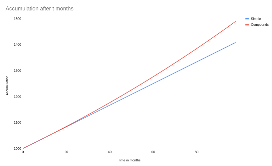
Figure 3.1: Interest Rate Comparison
5.3 Present and Future Values
The concepts of present value (PV) and future value (FV) are central to the time value of money. These two terms help explain the relationship between an amount of money today and an amount of money in the future.
5.3.1 Future Value
Future value refers to the amount of money an investment made today will grow to over a given period, assuming a certain interest rate. The future value is calculated using either simple or compound interest, but compound interest is far more common in practice and all subsequent formulae will follow the compound interest. The future value formula for compound interest is derived from the compound interest equation:
\[ FV = P \times \left( 1 + \frac{i}{n} \right)^{t} \]
Where: - \(P\) is the present value or initial investment, - \(i\) is the interest rate, - \(t\) is the time in years.
Future value helps investors or borrowers understand how much money they will have in the future based on a current investment or loan, making it a crucial concept in financial planning.
5.3.2 Present Value
Present value, on the other hand, is the reverse calculation. It answers the question, “How much is a future sum of money worth today?” Present value is essential when you are assessing investments or comparing cash flows at different points in time. The present value formula is:
\[ PV = \frac{FV}{\left( 1 + i \right)^{t}} \]
Where: - \(F\) is the future value, - \(r\) is the interest rate, - \(t\) is the time in years.
Present value allows you to discount future cash flows to their worth today. This is valuable for making decisions such as whether to invest in a project or how much to pay for a bond that matures in the future.
5.4 Discount Rates
A discount rate is the interest rate used to determine the present value of future cash flows. It reflects the opportunity cost of money—what you could earn if you invested your money elsewhere. The higher the discount rate, the lower the present value of a future sum of money.
Just as there are simple and compound interest rates, there are simple discount rates and compound discount rates.
5.4.1 Simple Discount
A simple discount is when a future sum is reduced by a fixed percentage to arrive at its present value. The formula for the simple discount is:
\[ PV = FV \times (1 - i \times t) \]
Where: - \(PV\) is the present value, - \(FV\) is the future value, - \(i\) is the discount rate (expressed as a decimal), - \(t\) is the time in years.
For example, if you are promised $1,000 one year from now, and the simple discount rate is 5%, the present value of that sum would be:
\[ PV = 1000 \times (1 - 0.05 \times 1) = 1000 \times 0.95 = 950 \]
In this case,$1,000 a year from now is worth $950 today.
5.4.2 Compound Discount
A compound discount works similarly to compound interest but in reverse. The present value is found by applying the discount rate to both the principal and the interest that would have been earned in previous periods. The formula is:
\[ PV = \frac{FV}{\left( 1 + i \right)^t} \]
Where: - \(PV\) is the present value, - \(FV\) is the future value, - \(r\) is the discount rate, - \(t\) is the time in years.
For instance, if you are to receive $1,000 in three years and the compound discount rate is 5%, the present value is:
\[ PV = \frac{1000}{(1 + 0.05)^3} = \frac{1000}{1.157625} = 863.84 \]
Thus, $1,000 in three years is worth $863.84 today at a 5% discount rate. Compound discounting, like compound interest, accounts for the effects of time and compounding, offering a more accurate reflection of the time value of money in many real-world applications.
##Yield Curves
Interest rates are not always fixed and can vary over the time period that an analysis covers. Yield curves provide a great way to understand expectations of future interest rates by various governments and banks. Using yield curves, rather than relying on constant or formulaic interest rates, provides several critical benefits. They give a dynamic view of the market’s expectations for interest rates and economic conditions over time. The primary benefits of using yield curves:
Reflects Market Expectations Yield curves show the market’s collective expectations for future interest rates, inflation, and economic growth. A steep upward slope in the yield curve often indicates that investors expect future interest rates to rise, possibly due to inflation or economic growth. Conversely, an inverted yield curve can signal a potential economic downturn, as it suggests that the market anticipates lower future rates, which are often associated with slower growth or recession.
Enhanced Decision-Making for Long-Term Investments Unlike a fixed or constant rate, yield curves provide rates specific to different time horizons (e.g., 1-year, 5-year, 10-year). This enables investors to make more precise evaluations of risk and return for bonds, loans, or investments with varying maturities. For example, when a corporation issues long-term debt, it can use yield curves to set interest rates aligned with prevailing market conditions, providing a more accurate reflection of future interest costs.
Better Risk Management Yield curves allow for more effective risk management by highlighting the term structure of interest rates. This is essential for managing interest rate risk, as different interest rate environments (e.g., a rising or flattening yield curve) can significantly impact the value of investments. Banks and financial institutions use yield curves to match assets and liabilities with appropriate durations, reducing the risk of unexpected rate changes.
Accurate Pricing of Products Yield curves allow for accurate pricing of various financial products, especially those with multiple cash flows over time. The ability to match each cash flow with the corresponding yield curve rate (rather than a single average or formulaic rate) allows for precise valuation and pricing that reflects real market conditions. This is crucial in structured finance, where products often have complex cash flow structures that depend on specific interest rates at different intervals.
Insights into Economic Conditions The shape of the yield curve is a valuable economic indicator. A normal (upward-sloping) curve often signifies healthy economic growth, while a flat or inverted curve can signal economic slowdowns or recessions. Policymakers, analysts, and investors closely monitor yield curves to gauge future economic conditions and potential monetary policy actions.
More Realistic Valuations and Discount Rates Yield curves provide a more nuanced approach for discounting cash flows, especially for long-term projects or valuations. Using a single discount rate, especially one that doesn’t account for changes in the economic outlook, can misrepresent the true value of a project or investment. Yield curves allow for the application of varying discount rates for each period, providing a more accurate present value calculation that aligns with expected market conditions. This is probably where the most value can be added to PA
Stress and Scenario Testing Yield curves allow for different options or views of the future to be adjusted to test for how base estimates change based on an unknown future. For example, a software purchase may add have a high ROI in a low interest enviromment, but no or negative ROI in a high interest one.
Dynamic Adjustment to Changing Market Conditions Yield curves are constantly updated, reflecting real-time changes in investor sentiment, central bank policies, inflation expectations, and economic indicators. Unlike a static, formulaic rate, the yield curve adjusts to market conditions and provides a timely measure of the current economic climate. This helps lenders and investors to remain agile in their responses to changing conditions, reducing the risk of using outdated or inappropriate interest rates in their calculations.
In a simple example, yield curves change the \(i\) in the formulae above to be time dependent. So, if we wanted to calculate the accumulation from above with 3 different rates instead of 1 constant rate, we would have:
\[ A = P \times ( 1 + {i_1})^{1/12} \times ( 1 + {i_2})^{1/12} \times ( 1 + {i_3})^{1/12} \] giving:
\[ \begin{aligned} \mathrm{A} &= 1000 \times ( 1 + {0.05})^{1/12} \times ( 1 + {0.045})^{1/12} \times ( 1 + {0.04})^{1/12}\\ &= 1000 \times 1.01187\\ &= 1011.87\\ \end{aligned} \]
While they may seem complex, yield curves are very easy to use and allow for assessments of the future that are more aligned to the the general economic views or to internal targets.
5.5 Why?
You may be wondering why all of this is necessary to know and how it applies to PA. Many analysts in PA use much of the theory above in calculating various rates. Another, more direct, application is when assessing the value of projects. PA professionals are often involved in assessing the value of software and other tech purchases for HR. I will dive deeper into these topics in a later chapters.